L6 Radiation
Module Description
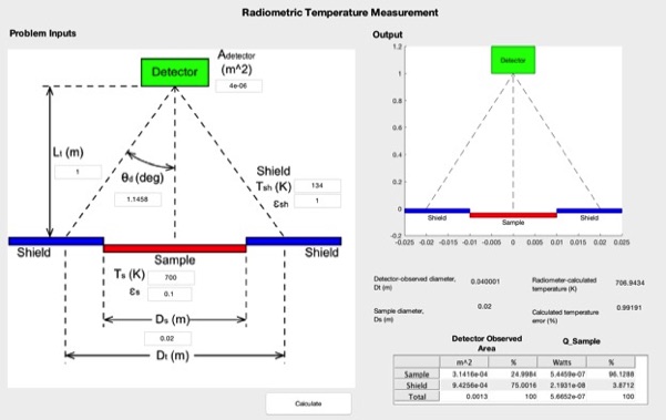
The radiation module simulates radiometric temperature measurement of an axially symmetric surface (disc) as observed from a radiometer detector. The disc is is guarded by an isothermal surface. Geometry and temperatures can be specified in order to compute radiometer-measured temperatures and radiation emission from surfaces as well as temperature measurement error as a result of radiometer acceptance angle and problem geometry.
Module Development Theory
Radiation Exchange - Theory
1. Overview
Diffuse, emitted radiation leaving a surface can propagate in all possible directions. Further, in the case of the detection of radiation emitted by a source, one must also consider the angle of observation (i.e. the angle over which the dector can 'see' radiation. Considering the case of radiation detection/measurement, one must consider the effects of the collection angle, as in the measurement of radiation emission from a surface, the detector-measured radiation emission is representative of all emission observed by the detector. Additionally, a radiation detector has a finite observation angle defining is obsesrvable cross-sectional area as a function fo distance from the detector and as such, sees a different volume depending on distance it is placed from the radiation source. . In taking a radiation measurement with a detector, uncertainty/errors can result from a number of sourcees, including (1) background radiation, (2) poor signal to noise. As such, the detection of radiation emitted from surfaces requires an understanding of how radiation propagates through space and how a detector's detection angle affects the cross-sectional area that is detected. The aim of this module is to investigate the effects of detector observation angle, standoff distance from sample, and background temperature on the overall magnitude of diffuse, hemispherical gray body radiation that a detector will observe as well as resultant temperature error associated with radiaitoncontributions of a background medium of a different temperature.
2. Mathematical Formulation
Radiation is emitted from all surfaces having a non-absolute zero surface temperature. There are a number of simplified models of radiation emission that are frequently used in engineering to describe emission from surfaces. While real radiation depends upon the angle of emission from a surface due to directional dependencies of emissivity (Fig. 1), it is frequently assumed that radiation is emitted uniformly in all directions (i.e. it is diffuse). If the emitter is also a flat surface, radiation emitted from the surface is said to be hemispherical and diffuse (Fig. 1). We frequently make the hemispherical diffuse assumption in order to simplify the calculation of emission quantities.

Figure 1. Diffuse vs directional emission (and absorption) from a flat surface.
We can draw additional insight into the process of radiation emission from simply phenomenologically considering diffuse radiation. In consideration of the diffuse emission described in Fig. 2, where rays of emitted radiation are shown, the total amount of radiation passing through a spherical shell of distance, r, from the emission point will be constant. However, due to the radial dispersion of emission, the density of radiation passing through a cross-section of area at a specified r decreases as r is increased. We term this emission density the emissive power, which is essentially a radiation heat flux passing through a spherical shell plane of distance r from the emission point. From Fig. (2), we define the solid angle,  , or in discrete form,
  , as
, as  .
.

Figure 2. Definition of the 2D plane angle (a) and its extenson to the 3D solid angle (b). Image modified from Bergman et al. [1].
In order analyze emission from a surface as observed from a radiation detector, we analyze the flat plate emitter, assuming axis-symmetry and that all radiation is diffuse. We additionaly neglect surrounding, environmental radiation, assume surfaces are gray. With these assumptions, the radiant power intercepted by the detector from within the hot disc 'target' area is
where  is heat flow to the detector,
  is the heat flow from sample disk to detector, and
  is the heat flow from the shield to the detector. The radiation contribution from the sample disk to the detector, using the solid angle, can be further written as
where  is the surface area of teh disc,
  is the inclination angle of the sample disc with respect to detector (zero radians),
  is the solid angle between the detector and sample disc, and
  is the sample disc emitted intensity, defined as
where  is the sample disc emissivity,
  is the quantity of blackbody emitted radiation from the sample disc, σ is the Stefan-Boltzman constant, and
  is the surface temperature of the sample disc. The solid angle between the detector and sample, , can be further defined using the definition of the solid angle as
where  is the detector area,
  is detector acceptance angle, and
  is the distance between the detector and the sample disc. Using (3,4), we can rewrite (2) as
Turning our attention to the contribution of radiation from the shield, we can write the contribution from the ring-shaped cold shield as
where  is the radiation intensity emitted from the shield,
  is the shield area,
  is the angle between shield surface and detector (the complement of ), and
  is the solid angle between the detector and the shield. Similar to the sample disc, the emitted radiation intensity from the shield can be written as,
where we assume the shield is black ( ). From the 2D geometry of the shield-detector, we can express area of the shield as
where  is the minimum of either the projected detector observation angle or mean diameter of the shield and
  is diameter of the sample disc. We can further express as
 , (9)
, (9)where  is the average of the sample diameter and the diameter of the radiation detector angle of collection at the sample plane. Note that in instances where the radiation detector collection angle diameter at this plane is smaller than that of the shield extent, we use the outer diameter of the shield here. More explicitly,
We can further define as
where R is the distance between center of the shield and the dector. We recognize geometrically that
We recognize then that we can write the heat transfer from the shield to the detector as
 . (14)
We can then solve for the total radiation reaching the detector from both the sample disc and the shield by using (5,14) in (1).
6. Putting it all together
The following is a default set of parameters which, when the included Matlab LiveScript .mlx file is run (script distribution), will execute the simulator.
area=4.0e-6; %m^2, detector area
Tsh=134.0; %K, shield temperature
emiss_sh=1.0; %emissivity of shield
Ts=700.0; %K, sample temperature
emiss_s=0.1; %emissivity of sample
Ds=0.02; %meter, diameter of sample
theta_d=1.1458; %degrees, the divergence angle of the detector
Lt=1.0; %meter, distance from detector to sample
radiation(area,Tsh,emiss_sh,Ts,emiss_s,Ds,theta_d,Lt);