External Flow - Theory
1. Motivation/Approach - Reduced Dimensionality of Convective Heat Transfer Coefficients
From development of the boundary layer equations, their simplification, and non-dimensionalization, the reduced dimensionality of the Nusselt number and convective heat transfer coefficient becomes apparent. Specifically, it can be shown that the average Nusselt number associated with external convective heat transfer to/from an object,  , is a function only of Reynolds number, Prandtl number, and object geometry. This redued dimensionality enables use of convection correlations in calculation and prediction of external flow convection. For additional details on the development of this idea, as well as development of the convective boundary layer equations, the user is refered to Chapter 6 of Bergman et al., "Fundamentals of Heat Transfer, 7th Ed.," Wiley, 2016.
 2. Direct Computation of Convective Heat Transfer
In solution of the 1-D steady state external flow convective heat transfer occuring from the surface of an object, we simply need heat transfer information about the geometry, the kinematic environment, and the momentum/thermal diffusive transport. In approaching the problem, we establish the kinematic environment (flow regime) through calculation of the Reynolds number, and momentum / diffusive transport through the Prandtl number, and employ correlations of the Nusselt number. More explicitly,
 (1)
(1) (2)
(2) (3)
(3)where V is the bulk fluid velocity,  is the hydraulic diameter of the solid object, ν is the kinematic viscosity, and α is the fluid thermal diffusivity. In computation of fluid properties used in determination of Reynolds and Prandtl numbers, properties are evaluated at the film temperature, which is the average of the free stream temperature,
  , and the object's surface temperature,
  . More specifically, for external flow heat transfer from cross-sections of regular shape (e.g. square cross-sections, circular cross-sections, high aspect ratio (thin) rectangular cross-sections, and inclined square cross-sections, as shown in Fig. 1., we can use the modified Hilpert correlation to calculate an average Nusselt number,
  (4)
(4)where  is the average convective heat transfer coefficient,
  is the thermal conductivity of the fluid,
  is the fluid Prandtl number at surface temperature condition, n is equal to 1/3, and C and m are geometry cross-section dependent coefficients, collected in Table 7.3 of Bergman et al. The valid domain on which the modified Hilpert correlation maybe used is geometry dependent. Generally, the correlation is valid for Reynolds numbers from
 Fig. 1. 2D regular cross-sections from which the simulator can calculate heat transfer. The dimension, D, is a characteristic dimension and an input within the simulator program.
From direct calculation of the average heat transfer coefficient, we can obtain convective heat flow to/from the cross-section per unit length as
 (5)
(5)where P is the perimeter of the cross-section.
3. Putting It All Together
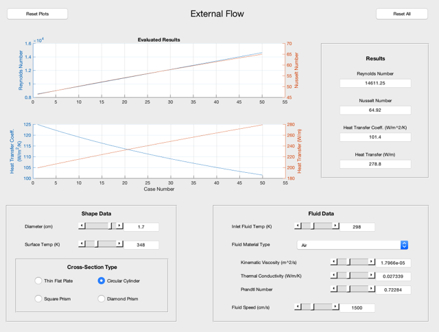
This procedure can be used to directly solve for convective heat flow using property lookup data for fluids knowing the geometry of the cross-section, the bulk fluid velocity, and surface and free-stream temperatures. The following set of code, when executed will execute the gui-based simulator with the provided set of input parameters.
Ts=348.0; % Surface Temp (K)
xsec=2; % Shape Index (1=flat plate, 2=cylinder, 3=Square Prism, 4=Diamond Prism)
Tinf=298.0; % Air Temp (K)
fluid=1; % Fluid Type, 1=air
v=1500.0; % Fluid Speed (cm/s)
plot_basic(d,Ts,xsec,Tinf,fluid,v);