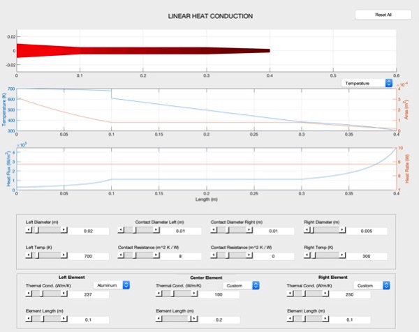
Module Description
The linear heat conduction module simulates one-dimensional, steady state heat transfer in the axial direction of an axis-symmetric composite solid. Exterior walls (radial direction) are insulated. The simulator allows control of boundary temperature conditions, thermal contact resistance, material properties of the three composite slab elements (preset or user-defined inputs), and allows control of the diameter of the slab element at each interface for simulation of a slab composite with a linearly changing diameter profile.
Module Development Theory
L1 Linear Condution
Linear Heat Conduction - Theory
1. Continuum Mechanics
Most physics problems can be broken down to the behavior of individual particles or atoms. This approach can be useful, but is usually far too difficult to handle directly. To speed things up, we try to characterize our problems by the averages of particle motion, where properties vary continously over the area or volume of interest. We call this approach Continuum Mechanics, and it's the backbone of not only heat transfer, but fluid dynamics, electrodynamics, strucural dynamics, and many others.
2. Control Volumes
To solve continuum problems, it's very useful to have a general "building block" that we can use to formulate solutions in a consistent way. One approach is to track batches of particles as they move, called Lagrangian Mechanics. Another, more common method, is to fix a control volume and analyze particles passing through, called Eularian Mechanics.

3. Continuity Equation
Properties like temerature, momentum, energy, mass or electric field can be defined for this control volume, and two things cause those properties to change in time:
- Material inside the volume changes, like chemical reactions or heat generation.
- Materials with different properties flow into or out of the control volume.
If we examine the case of energy (Q), we can construct a simple model of this behavior by stating:
Expressed for a volume, we can rearrange the terms and develop the follwoing expression
Where ( j ) is rate of change of energy at the surface, or flux. This expression is known as the integral form of the Continuity Equation. We can also use the divergence therorm to get a differential equation, also known as the Divergence Form:
4. First Law Revisited
Finally, we can use this equation to define the most important equation in heat transfer: the First Law of Thermodynamics! All we have to do is substitute heat  for temperature (T). We can use the equation
because no work is performed. Additionally, we can use Fourier's Law to define the flux term ( j ), which is the energy flow per area at the surface
Where k is the thermal conductivity. Subtituting these in for the Divergence form of the Continuity Equation, we get
which is nothing less than the First Law!
5. 1-D Linear Conduction
If we assume steady state and no heat source, we can reduce the Continuity Equation to the form
For a 1-D model with finite cross section, this becomes
For the derivative to be zero, the inside term must be constant, which indicates
Integrating this equation can then be performed
This formula, the Generalized Linear Conduction Equation makes no assumptions other than a constant thermal conductivity. We'll use this base equation to formulate solutions for several different problems.
6. Constant Area Conduction
Suppose we know the temperatures at the ends of a cyclindrical element  and
and  , with
  and
and  . If the cylindar has area
  and constant conductivity
  The generalized linear conduction equation can then be reduced
If we take a of constant cross-sectional area, we get
Using  , the constant
  can easily by found.
The remaining constant  can be solved for using the remaining boundary condition
Substituting back into the equation for  yields the final solution
Which corresponds to a linear change in temperature , as expected.
7. Contact Resistance
Along with the linear conduction equation, which describes heat transfer inside of an element, we need a relation to describe heat transfer between solid elements in contact wtih eachother. This is done with the relation for contact resistance, defined as
Where R describes how resistive the contact surface is. A high value of R indicates more resistance and a larger drop in temperature between the two surfaces. Note however, that this does not effect heat flow (q), which remains constant across the surface!
2. Linear Heat Conduction - Constant Area, Multiple Elements
By using our generalized conduction equation, and formula for contact resistance, we can now solve a rather intersting heat transfer problem. Shown below, we'd like to solve for the temperature profile acorss three elements, each with their own thermal conductivites, with temperatures fixed at either end. For now, we can assume constant area in all three elements.
1. Problem Solving Strategies
By far, the most challanging part of solving engineering problems is knowing how to approach the problem. It is often best to start by creating a list of information you know, and determine whether you really have enough data to solve the problem. Let's start with equations. We have many listed here, but many are too general or are copies of other equations. In reality, we have two useful equations
- Linear Conduction Equation

- Contact Resistance

The first describes temperaure inside each element, and the second describes the boundary between elements. If that's the case, then these equations, plus our knowledge of temperatures at the far left and far right should be enough to find a solution. The question we still have to answer though, is how do we stich these equations together and get a solution?
The answer is actually a general one, true for solving stress in segments of a beam, velocity segemetned into cells in a bounary layer, and ehat transfer in segements of cylnders. The solution is to devleop a series of equations that progress spatialyl from one end of the domain to the other, using only 1 additional unknown variable per eqch equation.
2. Variable Area Solution
We can now roll back our requirement of constant cross-sectional area. Starting with the general equation derived in part 6
We can develop an expression for area, assuming a linear slope in space
Using the same boundary conditions ( and ) we can eliminate by
Obtaining he expression for can be done by subtituting A(x) and integrating to the boundary condition
 (20)
(20) (22)
(22)Substitution into yields the solution
 (23)
(23) (24)
(24) (25)
(25)e (26)
(26)
(26)3. Putting It All Together
The above equation can be solve piecemeal for a three element experiment, with non-constant areas. The code below, when executed in the Matlab .mlx worksheet (download) will run the heat transfer simulator with the defined input values.
d=0.01; % meter
k=250.0; % Watt/(meter*Kelvin)
l=0.1; % meter
t1=1000.0; % Kelvin
t2=500.0; % Kelvin
r1=2.0; % Kelvin/Watt
r2=4.0; % Kelvin/Watt
plot_basic(d,k,l,t1,t2,r1,r2);