L2 Extended Surfaces
Module Description
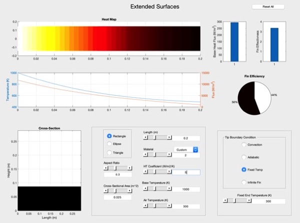
The extended surface module simulates steady state, 1-D conduction within an extended surface of regular geometry cross-section having convective heat transfer around the perimeter. The simulator performs calculations on rectangular, elliptical, and triangular geometric cross-sections of user-defined aspect ratio for various extended surface materials (preset or user-defined). A number of fin tip conditions may be utilized, and fin performance metrics (total fin heat transfer, effectiveness, and efficiency) are calculated.
Module Development Theory
Extended Surfaces - Theory
1. Overview
The term extended surface is used to describe a special case of conduciton in which heat is transfered within a solid within one direction and by convection/radiation at an object's surface in a direction that is transverse to the principle direction of conduction. A common example of an extended surface is a heat transfer 'fin' or a bank/array of fins to be used to enhance either cooling or heating of a fin/fin system's substrate. Fin systems are frequently used in cooling applications in which convective/radiative cooling of a surface itself is insufficient to enable operation of a heat generating device (e.g. a computer microprocessor). Fins come in a variety of different geometries and shapes. A few fundamental fin shapes are shown in Fig. 1.

Fig. 1. Diagrams of simple fin geometries, including (a) a rectangular fin of uniform cross-section, (b) a rectangular fin of nonuniform cross-section, (c) an annular fin, and (d) a pin fin of nonuniform cross-section.
2. 1-D General Conduction Analysis
As engineers we are primarily interested in knowing the extent to which particular extended surfaces or fin arrangements could improve heat transfer from a surface to a surrounding fluid. Consider first a single fin of one of the regular geometries shown below in Fig. 3. The determination of total heat liberated from a single fin requires analytical or numerical solution of the temperature distribution within the entire fin so that the total convective/radiative heat transfer from the fin's free surfaces can be calculated and summed. For the pin fin shown in Fig. 2, assuming that there is neglible radial temperature gradiant within the fin at any axial location, x, heat transfer within the fin can be treated to be 1-D in pursuit of surface temperatures of the fin. This drastically simplifies analysis and allows the determination of a closed, analytical solution to fin heat transfer.

Fig. 2. Arbitrary fin geometry and differential fin volume undergoing axial conduction and radial convection.
Considering a differential control volume at an arbitrary location, x, within the fin shown in Fig. 2, and assuming temperature within the fin is a function of x only, that is, T(x), and that fin cross-sectional area,  , is constant, we can write a control volume energy analysis for the fin as
where heat conducted into and out of the control volume are inidcated as  and
and  , respectively and
  is heat convected from the surface of the fin. We express as
Applying Fourier's law,
we can write (2) as
and expressing in terms of Newton's law of cooling,
we can substitute (4) and (5) into (1):
Letting  , where P(x) is the perimeter, (6) becomes
To perform integration, we change variables, substituting
into (7) to get
Equation (9) is the most general form of the extended surface heat transfer equation, with cross-sectional area, perimeter, and temperature all as functions of x. It can be solved numerically using 1-D finite difference techniques.
3. Analytical Solutions Assuming Uniform Fin Cross-section
For the special case where  , (9) reduces to
the solution to which is
where constants are determined by a constant temperature left hand boundary condition, that is that the temperature at the base of the fin is equal to the base temperature,  , along with four possible fin tip boundary conditions: (1) convection at the fin tip, (2) an adiabatic fin tip, (3) a perscribed temperature fin tip, and (4) an infinitely long fin. Fin heat flow rate can be calculated from application of Newton's law of cooling at x=0,
Particular solutions to the temperature distribution (11) and the total fin heat flow,  are tabulated in heat transfer texts (e.g. Ch. 3 of Bergman et al., 7th Ed.
4. Validity of the 1-D Extended Surface Analysis
Given the multi-dimensionality of an extended surface problem, a 1-D analysis is often applied to such problems. Valid application of a 1-D analysis requires that the problem have negligible temperature gradient in the directoin perpendicular to axial conduction.
5. Putting it all together
The following is a default set of parameters which, when the included Matlab LiveScript is executed (script distribution), will execute the simulator.
h=0.1; % Convective Heat Transfer(Watts/(meter^2*Kelvin))
area=0.025; % Cross-section Area (meter^2)
ar=0.1; % Cross-Section Asepect Ratio
l=0.2; % Length (meter)
k=2.0; % Material Conductivity (Watts/(meter*Kelvin))
tbase=1000.0; % Base Temp (Kelvin)
tair=300.0; % Air Temp (Kelvin)
cross_section=1; % Set Cross Section to Triangle
tip_bc=3; % Set Tip BC to convective
plot_basic(h,area,ar,l,k,tbase,tair,cross_section,tip_bc);